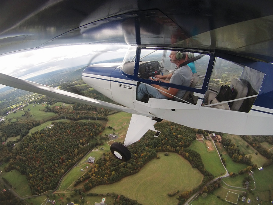
“It doesn’t take long to fly 40 hours,” said my local friend. “You can fly two hours in the morning, two hours after lunch, and that’s six right there.” The fellow that gave me this advice was joking, mostly. This was among the advice that I received while preparing to start Phase I testing on the four-place Bearhawk that I had been building over the past four years.
It takes effort for me to avoid a visible cringe when I hear a builder talk about “flying off the hours” on a new homebuilt airplane, implying that the 25- or 40-hour test period is just a time to go fly solo for a while, boring holes in the sky as quickly and cheaply as possible. Regulators specify their requirements for Phase I testing, and prudence and personal responsibility add on a few more. The test period is an opportunity to get some very important things done to make sure that the airplane is as safe as we are expecting it to be, but how is an amateur builder to make the most of that opportunity? Some builders are trained flight test engineers, but I’m not one of them.
In initial flight testing, builders and test pilots have at least two main responsibilities to ourselves, our future passengers, and any future pilots or owners of our planes. One is to experience the entire envelope of speeds, load factors, weights, and CG range to discover any lurking bad habits. Vaughan Askue’s Flight Testing Your Homebuilt Airplane is a great resource for how to do this safely, as is FAA Advisory Circular 90-89A, Amateur-Built Aircraft and Ultralight Flight Testing Handbook.
The second main responsibility of Phase I testing is to create a means for predicting airplane performance in various environmental conditions. In operational use, these predictions will help us know if we will be able to clear the trees at the end of the runway, or climb over the mountains along the route, for example. I’ve personally had the miserable experience of beginning a takeoff roll in a type-certificated light plane and not being sure that I’d have enough of a climb rate to stay safe in the initial climb. I was pretty sure, but I was flying a very old airplane with a very thin POH, and I didn’t have any way to be certain. This is an experience that I never want to repeat, especially not with an airplane full of wife and kids.
Flight testing was easy for the first few hours. I found plenty of guidance about how to plan and safely execute the first and second flights. After a few hours of envelope validation, it was time for me to start thinking about performance prediction, and I didn’t have a plan that I was excited about. I could go fly and establish parameters like VX, VY, and their corresponding rates of climb for one flight, but how would I extrapolate that data into numbers that would apply on days that were hotter or colder, with an airplane that was heavier or lighter, or at a density altitude that was higher or lower than the original condition? How would I establish a functional upper safe density altitude limit without conducting risky operations at hot and high airports? Surely there must be a way to derive these results without having to experience them all and record the results.
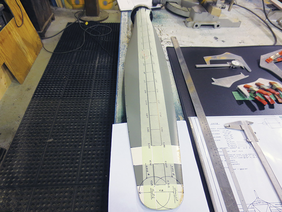
Finding the total activity factor (TAF) for the prop required making marks at calculated intervals and entering the chord measurements at those marks into one of the Bootstrap spreadsheets.
Check AVweb
A bit of Google searching led me to a series of articles (“The Bootstrap Approach to Aircraft Performance”) in the AVweb.com archive by Dr. John T. Lowry. Dr. Lowry created a mathematical model for predicting airplane performance in a wide variety of situations, based on inputs from a small set of test flight data. He refers to this as the Bootstrap method. The AVweb.com articles are the “CliffsNotes” version of the model, though the full version (complete with mathematical derivation) appears in Lowry’s Performance of Light Aircraft. This is a fantastic, but currently unobtainable in print, 475-page book published by AIAA in 1999. I found his method to be exactly what I was looking for, and I don’t know why everyone else isn’t using it, too. Here I’ll explain how I have been able to apply his method to my flight tests, and provide suggestions for how you can do the same.
The first step is to find and read the articles in the AVweb.com archive. Do a Google search for “Bootstrap AVweb,” or enter “Bootstrap Approach” in the search box at the top of the page at www.AVweb.com, and you’ll find one of the three articles. Read at least the first two articles, and download the associated spreadsheets:
I used Excel to open the sheets, but they are fairly old and will likely be compatible with other programs as well. The first article and spreadsheet cover performance of airplanes with fixed-pitch props, and the second set covers constant-speed props.
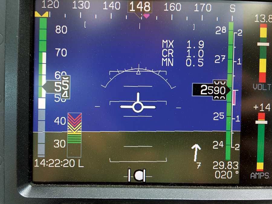
Note that the airspeed is steady at 55 knots with no trend indication. Watch the pitch angle to look for the earliest indication of deviations that will show up in the airspeed a few seconds later.
Collect Data
The process for using Lowry’s method is to collect the data to complete the “Bootstrap data plate.” As he points out, the easy numbers are wing area and span, rated power, rated rpm, and prop diameter. These are easy because we can just look them up or measure them, assuming we don’t already know them. The slightly harder tangible measurement was “Z,” the ratio of fuselage diameter to prop diameter. In the Bearhawk the diameter measurement falls right around the middle of the cabin, so it would have been easier to measure before the wings were on. Fortunately the fuselage is mostly square in that section, so it was not hard to measure around the wing and approximate a fairly accurate total perimeter.
Since I’m working with a constant-speed prop, I had to find the total activity factor (TAF), which the spreadsheet calculates from my measurements of the prop. I stretched a piece of masking tape from the tip of the blade to the spinner of our 76-inch Hartzell prop, as close as I could get it by eye to the middle of the blade. I took my computer to the hangar and used the top section of the second spreadsheet to make marks at each 1.9 inches, measuring from the tip inward. The spreadsheet even does the math to tell me how those 1.9-inch increments add up, and what the sum is in whole inches and sixteenths of an inch, since that’s how most of our rulers are calibrated.
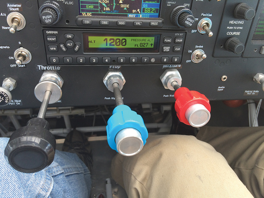
At first it felt strange flying with the prop control all the way back. The engine runs fine in that configuration, as long as the throttle is at idle.
Fly the Plane
The rest of the data plate numbers come from flight test results. These gliding and climbing tests should come after airspeed indicator calibration tests. If you have trouble finding a way to do those, Dr. Lowry offers an expanded set of Bootstrap spreadsheets for sale, and one of those extra spreadsheets has a handy tool for using GPS groundspeeds on three different headings to easily find airspeed errors. I only needed to record the gliding tests, so I flew glides at five-knot increments from 45 to 70 knots while descending through a 500-foot window. I made an effort to shuffle the speeds around so that gradual environmental changes of the warming morning wouldn’t skew only one side of the data. For example, I didn’t fly the glides in order starting at 45 knots, but rather one at 60, one at 45, one at 70, etc.
I would usually start the descent at least 100 feet high as to be well-stabilized during the window. I could maintain the test speed within a knot if I used the attitude indication on the EFIS as the primary pitch information, since pitch deviations were obvious there, long before they showed up in the airspeed indication. I disregarded data on runs where I saw that my technique caused speed variations of more than one knot. On more than one occasion, I ended a glide test early and started climbing for the next one because I knew I wasn’t stabilized enough to get good data. This is one part of Phase I testing that would have been safer with an observer to help look for traffic, since I found myself focusing much more on inside cockpit references than an outside traffic scan. This is something to consider if you’ll be applying these techniques to an airplane that is not restricted to one occupant.
As Dr. Lowry instructs, I flew these glide tests with the engine idling and the prop control all the way back. I had not tried bringing the prop control back in flight before, but it was interesting to see the rpm drop from the normal 1100 rpm idle to be closer to 690. The engine was smooth in this condition, as long as I didn’t advance the throttle much above idle.
My glide times were always right around a minute, ranging from 50-60 seconds. Lowry’s first spreadsheet has a handy calculator for processing the glide tests, but it is hiding over on the far right side in columns AA through AK. I used those tools to find the parasite drag coefficient and the airplane efficiency factor. It is important to remember that the best glide speed occurs at the minimum of the product of the airspeed and the glide time, not the minimum glide time. The latter represents the minimum sink speed, which is going to be slower than best glide by around 30%.
Work the Numbers
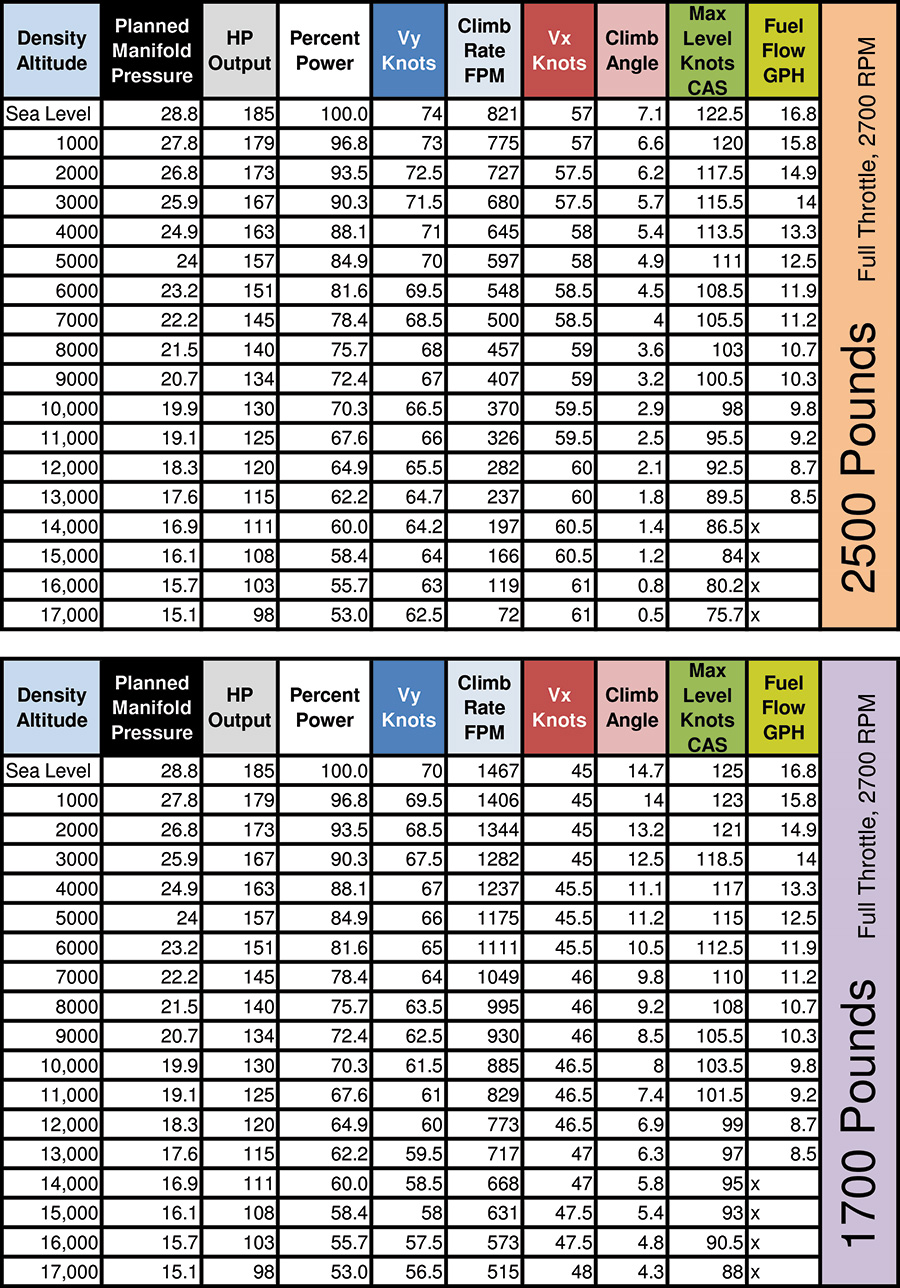
With the data plate complete, I started tinkering with the operational variables in cells B77 through B80. These include actual gross weight, actual density altitude, actual rpm, and percent of engine power. I used a Lycoming engine chart to find the actual horsepower at different altitudes and power settings, and then made a chart of my own that shows the percentage of horsepower for each of those conditions (see the white column header in the climb charts above). For example, if I want to consider a full-throttle, 2700-rpm condition at 6000 feet density altitude, I need to know that the engine is only going to be producing 151 horsepower, or 81.6% of the max-rated 185. As the density altitude climbs, the maximum percent of horsepower available obviously decreases, so it is important to remember this reduction. Upon completing those four operational values, the spreadsheet returns the expected performance in cells D87 through F91 that include the maximum level speed, VY in knots, rate of climb at VY, VX in knots, the angle of climb at VX, best glide speed, angle of glide at that speed, minimum sink speed, and rate of sink at that speed.
I found by experience that it was especially important to put a meaningful number in cell B102. This number is the lowest airspeed that the model considers when it calculates all of those optimum speeds, and is set to 60 by default. I made a chart of optimum speeds at low gross weight and the numbers weren’t making sense. VX was 60 in all cases, and VY reached 60 long before the absolute altitude. Astute pilots will recall that VX and VY (in fact, all speeds) converge at the absolute ceiling. The problem was that my true VX was more like 45 knots, but since 60 was the lowest airspeed the model was considering, that speed yielded the most optimum climb angle, so it labeled 60 as VX. It wasn’t exactly incorrect, since the climb angle at 60 was better than the climb angle at 61, but like any other computer model, bad user input was leading to bad results. The takeaway here is that users should be sure to change the value of B102 to something close to the lowest stall speed to be sure that the actual VX will be somewhere in the chart. The remaining speeds in the subsequent rows of the B column will automatically populate to half-knot increments above the value of B102.
Chart the Results
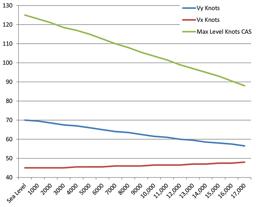
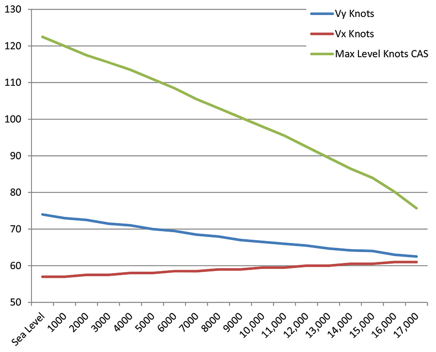
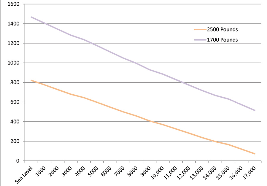
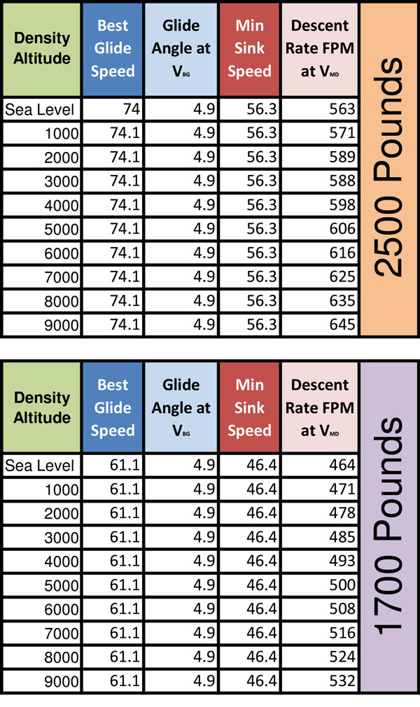
I created the charts shown here by combining the Lycoming chart data and the second of Lowry’s spreadsheets. In the climb charts, the second, third, fourth, and last columns contain data from the Lycoming charts, and the remaining columns are from the Bootstrap model. The glide charts are based entirely on Bootstrap calculations, since the engine is not a player. These charts are useful for case-by-case reference, as well as for developing mental rules of thumb. For example, note in the 2500-pound chart that my climb rate is going to be less than 500 feet per minute starting at around 7000 feet density altitude. This is a handy density altitude to keep in the back of my head, since I know that a climb rate of less than 500 feet per minute is below my comfort zone in most operations. It is worth noting that at a solo, half-fuel weight of 1700 pounds, this 500 fpm red flag occurs at just over 17,000 feet density altitude. I mention that just in case you were wondering how important weight is in airplane performance.
There are endless possibilities for creating charts like these. I used 1700 pounds and 2500 pounds because those are the end points of my normal gross weights, but it would be possible to create the same type of chart for other intermediate weights. The Bearhawk is a very straightforward and forgiving airplane, so when it comes to making operational decisions, it just hasn’t been too important for me to make precise interpolations. In most cases even the worst-case numbers are good enough for what I’m doing. The line graphs are based on the climb charts, and the shape of the curves shows the convergence of the three speeds as altitude approaches the maximum.
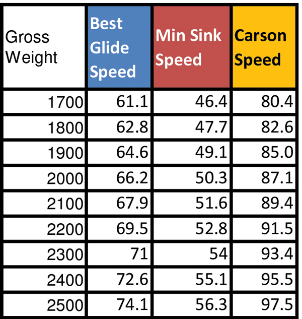
Best glide speed, minimum sink speed and Carson speed at various gross weights. Carson speed is the sweet spot where the least amount of fuel is used for significantly greater speed. It is named for B.H. Carson, the aerodynamicist who identified it.
If we think of the aforementioned charts as a means of populating an operating handbook, the Bootstrap method is also very useful for understanding how the different environmental factors impact performance. For example, consider a scenario where the density altitude is 5000 feet, weight is 2000 pounds, and the wide-open-throttle engine output is 157 horsepower, or 85%. The model predicts a maximum rate of climb of 915 feet per minute at a VY of 67.5 knots. If we were to make an imaginary modification to the engine that gave it an extra 20 horsepower, but weighed 200 pounds, would that make for a net gain in performance? If we increase the horsepower to 73% (135/180), the climb rate jumps to 1066 feet per minute. Increasing the weight to 2200 pounds reduces the climb rate back down to 914 feet per minute. How interesting-in this particular case, there is no net gain in climb rate.
It is easy to spend a whole afternoon tinkering with the numbers. I recently used the propeller measurements from a fellow-builder’s 80-inch prop to create a blade activity factor for his prop. I created a copy of the second Bootstrap spreadsheet and added his numbers to run similar scenarios. His larger prop yielded better performance on climb rate and top speed, but the differences were too small to be measurable on all variables except absolute ceiling. The larger prop provided for an extra 1000 feet or so.
Best glide speed, glide angle, minimum sink speed and descent rate at various density altitudes and 1700- and 2500-pound gross weights.
Something for Everyone
The model is applicable to any airplane at any phase of testing. If you have a few hundred hours in your homebuilt, but don’t have the kind of detailed performance predictions that you’d like to have, grab a friend with good traffic-scanning skills and go get some data. The same applies if you regularly fly a normal-category airplane that might have been made before the days of the GAMA standardized POH.
It is important to remember that these numbers are all based on calculations and not actual tests. I happen to think that the calculations are pretty close, and my actual performance has been very close to what the model predicts. The accuracy of the model’s predictions are going to depend primarily on the accuracy of the inputs to the Bootstrap data plate and the operational variables. There is inevitably going to be some scatter in the data, but I found that in an airplane like the Bearhawk, the scatter was small enough to be operationally insignificant. As Lowry points out in his book, the curves of these equations are relatively flat in GA airplanes, so the model is fairly forgiving of small variations. I was glad to have found Dr. Lowry’s work when I did, and I hope you’ll find it useful and share your results, too.

