 In previous articles in KITPLANES® (October 2018, May 2019 and July 2019), I outlined the premise of an adjustable tuned-induction system. As a quick review, the point is to be able to optimize engine function by increasing its volumetric efficiency for greater horsepower and/or economy by runner wave timing. That’s done by being able to individually adjust all the runner lengths so that the wave propagation in the induction runners can be equal and timed for the engine’s benefit. So, you must be able to have a way to adjust the runner length to optimize power output at the targeted rpm.
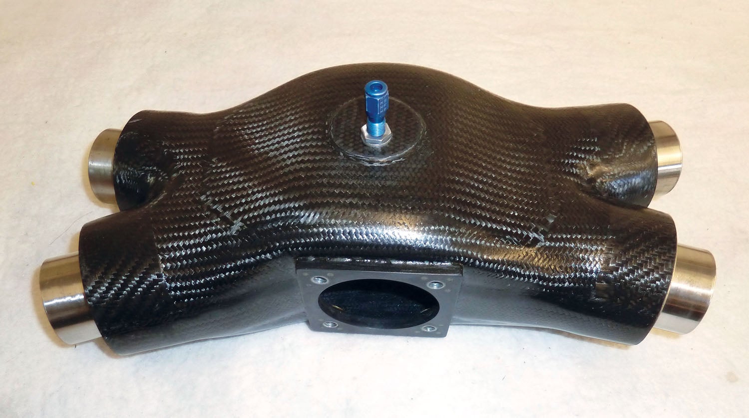
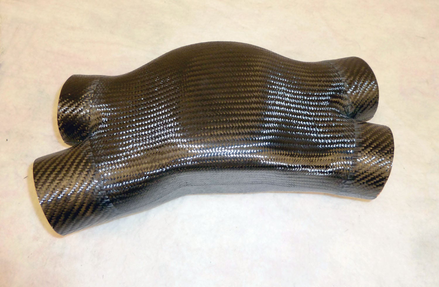
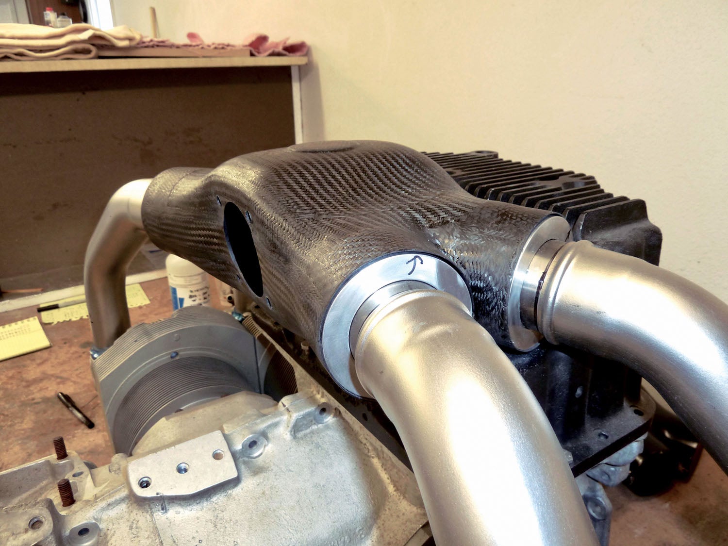
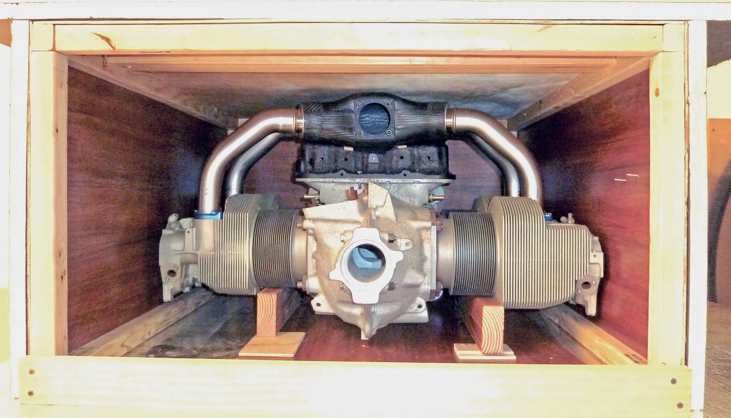
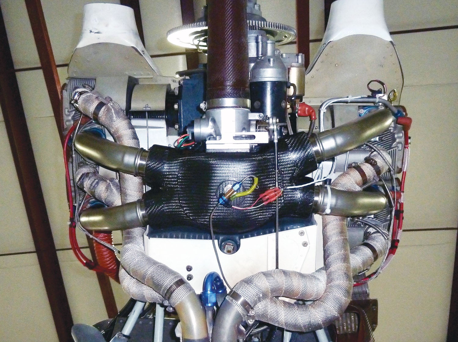
A key component of the induction system is the plenum. Made from carbon fiber and high-temperature resin, it was designed to fit the fixed dimensions on the engine and space available under the cowl. It also had to be compatible with existing Sky Dynamics induction components.
Fabrication
As it turned out, this plenum is the most difficult project I’ve ever attempted in composite. I’m certain that composite builders are scratching their heads and wondering, What’s so difficult about building a plenum? For the uninitiated, let me explain:
Composite work is a discipline that requires more planning and time organizational skills than most metal-plane builders are used to. A metal-plane guy just goes out to the shop and drills something, deburrs it and then drives a rivet into it. Well it’s actually a bit more difficult than that.
However, a composite builder has to know exactly what he is going to do during a work session. He has to make certain all the materials are ready, cut all the patterns in advance, plan the layup and then make certain there’s enough manpower and time for the job at hand—not to mention the incessant itching.
But in this case, there was even more: Before I could build the plenum, I first had to make a simple, inexpensive shop oven to cure the high-temperature resin (see the May 2019 issue for details). I also ran a few tests to familiarize myself with the new materials required for the project. After a bit of trial and error, I was ready at last to tackle the final plenum.
While developing the final configuration of the plenum, I was able to increase the volume of the plenum to 190.98 cubic inches. This allowed a decrease in the amount of mean pressure drawdown during the piston’s intake stroke. If you can decrease the amount of drawdown, there will be a higher mean pressure in the plenum for cylinder fill.
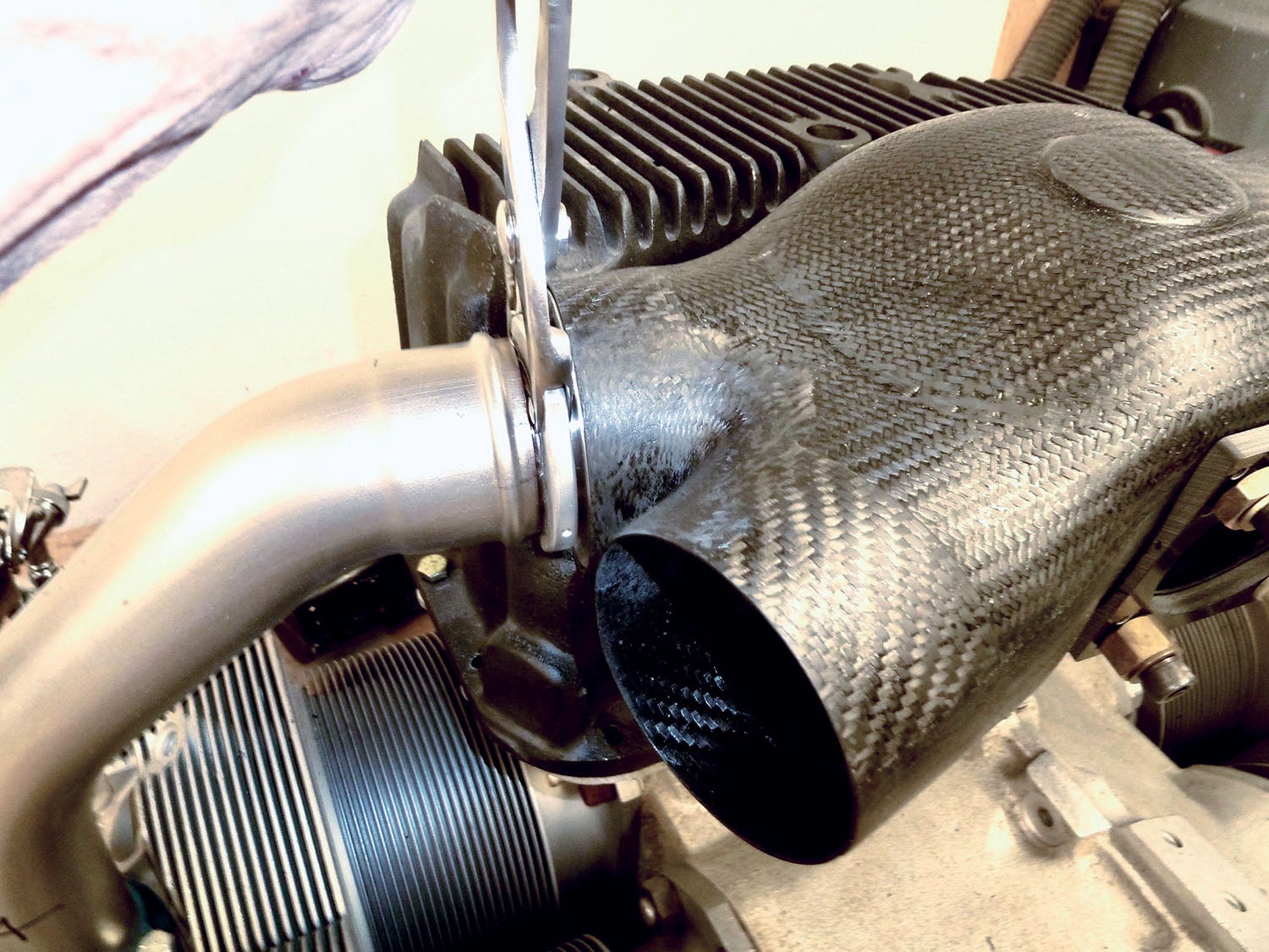
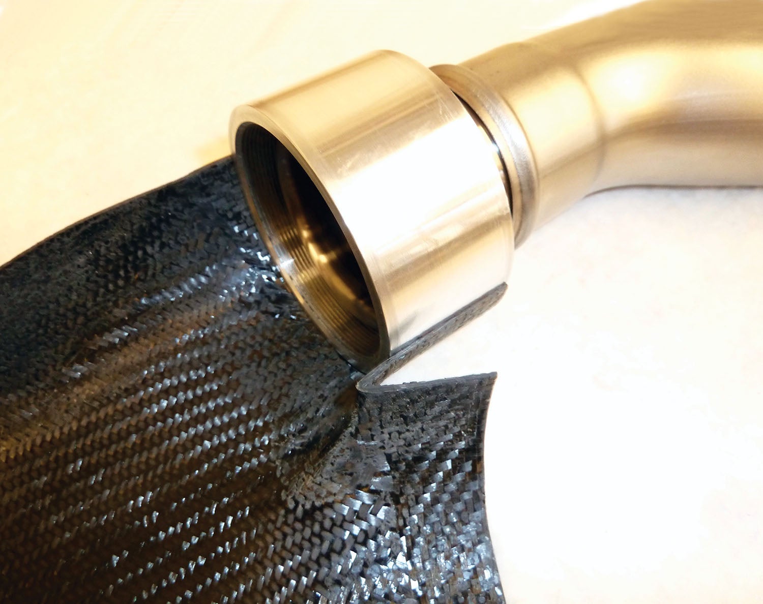
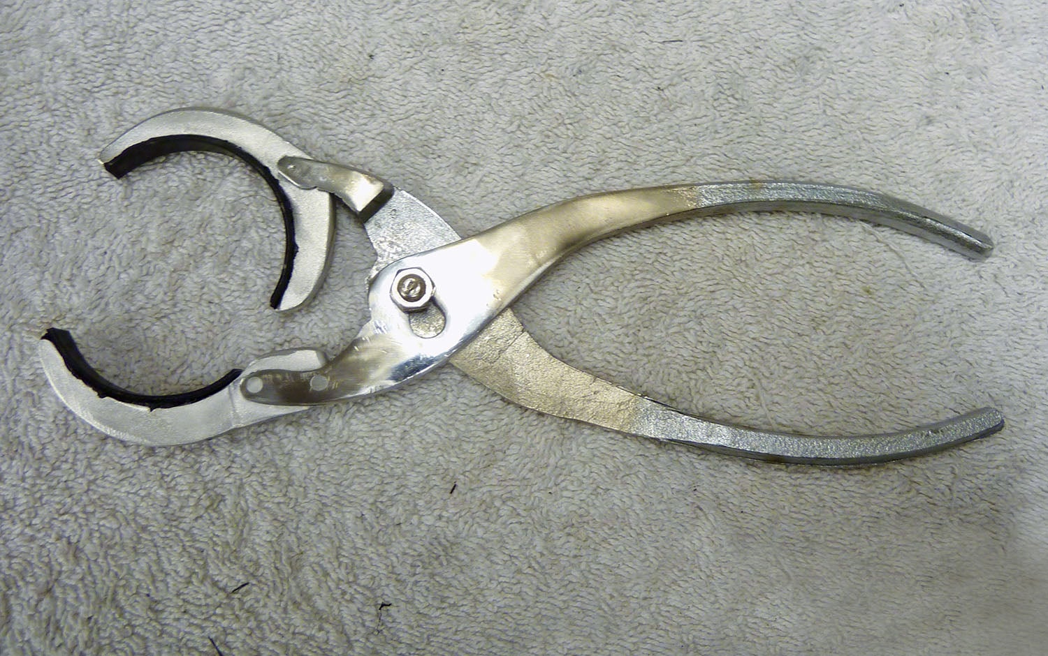
A simple type of homemade oil filter wrench was fabricated from old pliers to allow the runner to be adjusted. Between the carbon fiber plenum and runner, there is about 3/8 inch of the exposed portion of the adjustable velocity stack. O-ring seals are on both sides of the exposed portion. The load from the two O-rings on the velocity stack makes it difficult to turn and holds its position during engine operation. Each revolution of the velocity stack changes the runner length 0.050 inch.
Next, the threaded sleeves were bonded into the plenum ports by using the prescribed bonding technique. Since the final bonding of the threaded aluminum sleeves into the carbon fiber plenum must be extremely accurate, the entire engine assembly went into the oven.
Testing
Our goals were to be able to tune the induction runners to each cylinder, possibly have a little less manifold absolute pressure (MAP) drawdown with each intake cycle, and eventually be able to harness Helmholtz resonance.
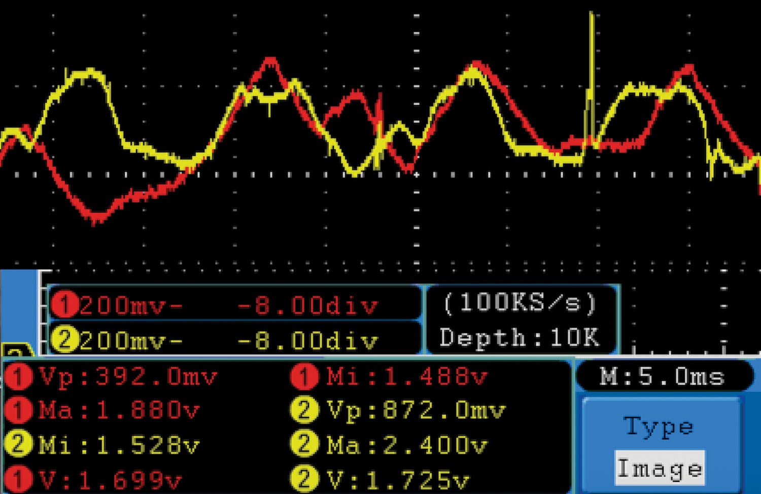
We discussed wave propagation in the May and July 2019 issues. The oscilloscope trace in Figure 1 represents 720° of crank rotation and was the last test of the original plenum at 2830 rpm, 27.6 inches MAP, 3860 feet pressure altitude, 60° F outside air temperature and 242 mph.
This trace is 200 millivolts per division. Looking at the yellow plenum pressure trace, at first glance it’s obvious the four inlet cyles depicted in the graph don’t look as if they’re very symmetrical across the trace. This is due to the original unequal runner lengths. The lowest point of the yellow trace represents the lowest pressure in the plenum due to drawdown during the intake cycles. The highest point presents the maximum plenum pressure recharge due to q (free stream dynamic pressure).
On the left side of the graph, the yellow line shows around a 3-millisecond lag before the plenum begins to see the pressure drawdown from the piston during the intake stroke. Then the plenum catches up with the cylinder fill rate and repressurizes the plenum at q minus induction losses. Then about 3 milliseconds later the pressure in the plenum begins to rise with a pressure recovery that is faster than the cylinder fill rate (under these engine and flight conditions) until it reaches the plenum’s maximum pressure.
What you also can see is that the pressure at the back face of the valve is greater than the maximum pressure in the plenum (the same calibrated sensors are used at the head and plenum locations). So that’s the minimum and maximum pressures represented in the trace.
But what about all the other odd yellow shapes? If you can imagine, at this rpm (2830 rpm) the wave propagation in the intake runner from IVO (intake valve opening) to about 40° before the IVC (intake valve closes) makes about three round trips (3N) from the valve to the plenum and back. Then that leaves about five round trips (5N) that occur after the IVC until the IVO again. So there are about eight round trips (8N) per cylinder in 720°. That means there are a total of about 32 round trips (at this rpm) in my four-cylinder engine during this time that is seen by the plenum sensor.
Since the intake runners aren’t the same length, each set of 8N from each cylinder is at a different frequency. The plenum sensor is recording four sets (each cylinder is a set) of different frequencies, and remember they’re also attenuating with each N trip, which will give you a very strange summary wave pattern as the sine waves go in and out of phase from each runner. Howard Claiborne, who has contributed much of the engineering expertise in wave propagation to this project, and I were hopeful that the FFT (Fast Fourier Transform) will let us see the wave propagation frequency of each runner.
Now, back to what information we can see in the plenum trace. The maximum to minimum pressure variation at the intake valve (red trace) was .392 volts or 5.69 inches Hg. The plenum (yellow trace) experienced a .245-volt pressure variation for 3.55 inches Hg, while the Dynon indicated a mean pressure of 27.6 inches MAP. During the same time, the runner pressure at the valve varied from 25.14 inches to 30.83 inches. The fact that the valve experienced a lower pressure than the plenum is due to the proximity of the piston drawdown force and the volume ratio of the cylinder to the local volume of the runner. The higher pressure at the valve than in the plenum is due to the energy in the mass flow momentum in the runner.
So, what is all this for? With my original plenum and unequal runner lengths, while the plenum mean pressure was 27.6 inches MAP indicated on the Dynon, the maximum pressure at the back of the intake valve was 30.83 inches. That’s an increase of 3.23 inches at the back face of the valve over the indicated MAP under these conditions. This is due to air-column momentum, runner-tube taper and wave timing. The wave timing in my original plenum may not be contributing and may in fact be hindering the maximum pressure achievable in the runner at the valve.
What we want to achieve is maximum pressure in the runner at around 40° before the IVC. This will result in maximum cylinder fill and thereby increase volumetric efficiency (VE).
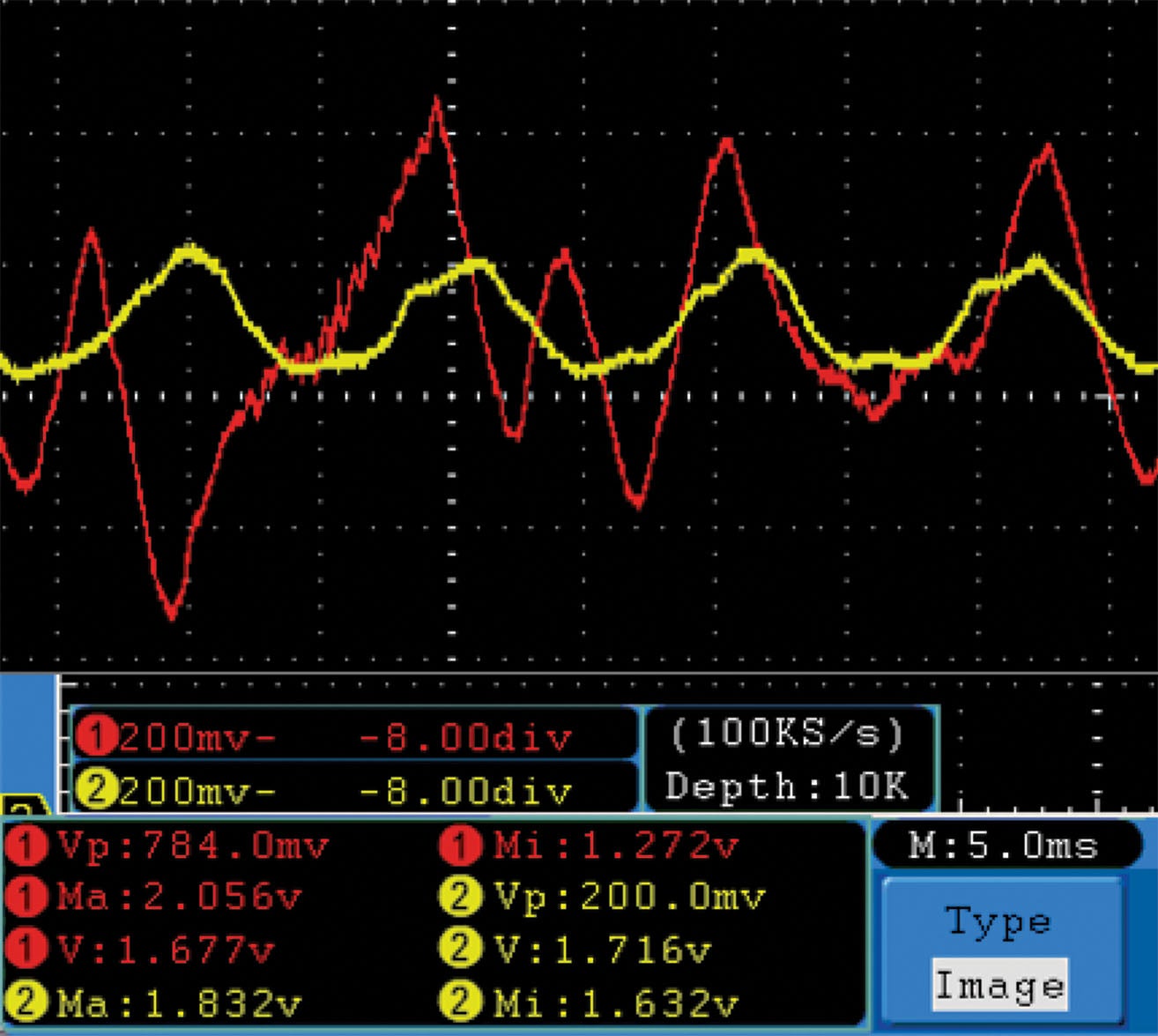
Figure 2 shows 720° of crank rotation during the first test of the new adjustable-runner tunable carbon fiber plenum at almost exactly the same test conditions of 2830 rpm, 27.7 inches MAP, 3860 feet PALT, 60° F OAT and 242 mph.
The oscilloscope is set exactly the same as in Figure 1. The yellow plenum trace is obviously more symmetrical, so the runners are nearly the same length and the wave forms from each cylinder are closer in shape. Although they may not be perfectly tuned, they’re close.
The maximum to minimum pressure variation at the intake valve (red trace) was .784 volts or 11.38 inches Hg. The plenum (yellow trace) experienced a .200-volt pressure variation for 2.9 inches Hg, while the Dynon indicated a mean pressure of 27.7 inches Hg MAP. During the same time, the runner pressure at the valve varied from 22.01 inches Hg to 33.39 inches Hg.
The larger volume plenum had less pressure drawdown as there is more volume in the plenum to increase resistance to the effect of the piston swept volume during intake. So 3.55 inches – 2.9 inches = 0.65 inch less drawdown in the new plenum. This means plenum pressure increased 0.325 inch.
Let’s use the same formula (rule of thumb) we’ve used before:
(2.1 hp/cylinder/1-inch increase in MAP) x .325 inch x 4 cylinders = 2.73 hp
Notice the lowest pressure at the valve dropped 3.13 inches more than it did with the original plenum. That’s because the runners are longer and the piston has more effect in drawing down the local pressure at the valve as it gets the energy in the runner to start moving the larger (longer) air column. However, even more importantly, it reached a maximum pressure at the back of the valve of 33.38 inches Hg, which is 2.5 inches Hg more than the original plenum.
So in this situation, the valve is experiencing about 5.68 inches more than the Dynon indicated plenum pressure. Now, if we can time that by adjusting the length of the runner so the maximum pressure occurs at the optimum time for maximum cylinder fill, we can increase the volumetric efficiency of our engines.
Results
1. Larger plenum volume produced lower pressure drawdown in the plenum and therefore a higher mean plenum pressure and about 2.73 additional hp.
2. The more the runners are the same length, the more similar the propagation wave forms are, as is apparent in the oscilloscope trace of the new carbon fiber plenum (Figure 2).
Now for the bad news. Howard and I have run traces for a year now, perhaps more than 80–100 of them at varying engine parameters. Howard made a spreadsheet of the harmonics of the engine, so we were pretty certain of the Hz range that we are looking for. There are also engine functions at specific rpm that may obscure the wave propagation frequency in the induction runners. Mathematically, we should be able to calculate the wave propagation Hz with the speed of sound we have at our induced air temperature (IAT).
Wave Hzs = C / 4 x (Leff)
Where:
C = Speed of sound at induced air temperature.
Leff = Effective length of runner = runner measured length + 0.5 x average runner diameter.
This would be a runner wave frequency around 171 Hz, so the pulse we are trying to see at the sensor in the induction plenum would be two times that, or 342 Hz, which is the wave round trip to the plenum (also called the N number). However, it may be blanketed at some rpm due to the sound produced from some of the engine events like valve openings. So we may not see the runner wave Hz at those specific rpm, but by varying the rpm of the engine a bit the Hz of engine events would change and the wave runner frequency wouldn’t. So, it should be visible in the FFT, right? We started looking for the frequencies where we thought we should see the runner Hz, and we did not see a thing. Bummer.
The previous paragraph took Howard and I months to figure out. (Isn’t experimenting fun?) Then it dawned on us that we are looking for the frequencies on a 4-cylinder horizontally opposed engine, and the closer we get the runners tuned, the less we will see that wave frequency since literally 180° later, the same frequency is being generated in a different cylinder at the same amplitude, which should produce an algebraic summary wave of “0,” just like a noise-cancelling headset. Unfortunately that is exactly what we saw: nothing! It seems now that we should have known that already.
What to do next? After more than a year and many, many hours of testing, we proved that we can’t do more than empirical evaluations. I don’t mean to diminish how important those observations are, but from a scientific standpoint we couldn’t prove all we wanted to when we set out with this premise. We knew it worked but how much? We already knew that at the same AFR (air-fuel ratio) with the original plenum, testing showed we had already increased the efficiency 4.5% with the new plenum even though it isn’t perfectly tuned yet.
Ricardo Software to the Rescue
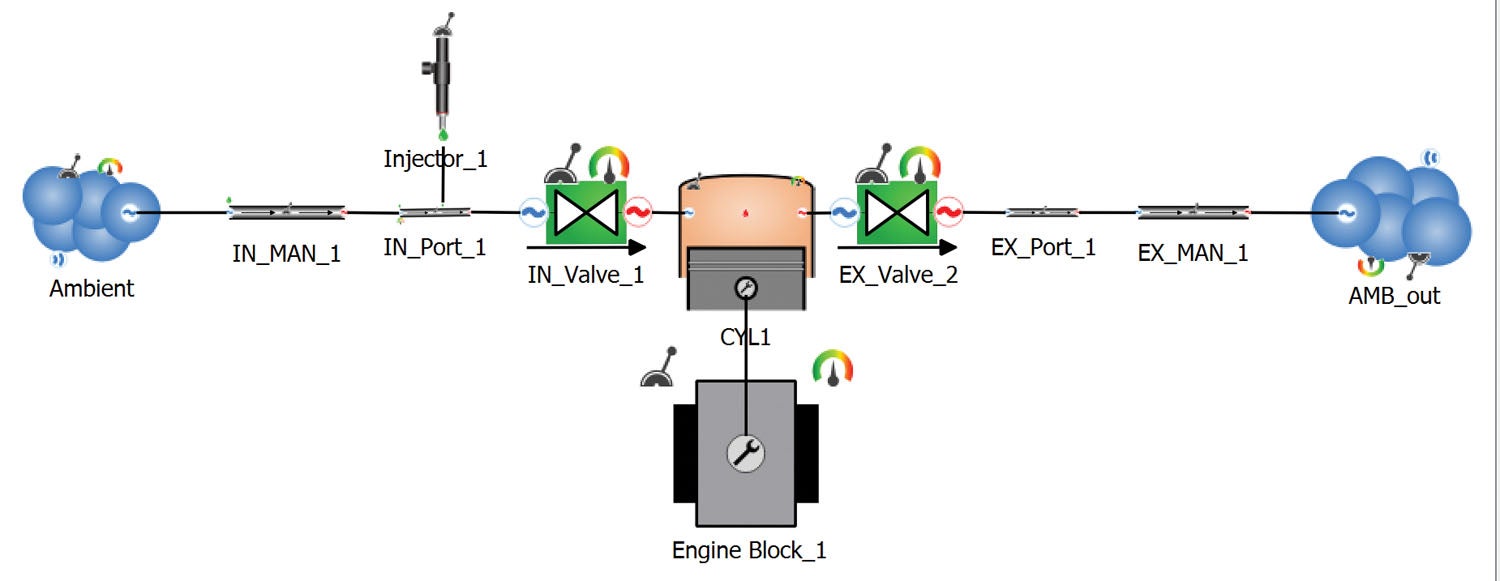
Ricardo WAVE is the leading ISO-approved 1D gas dynamics simulation tool. It produces steady-state performance simulations for almost any engine configuration validated with 98% accuracy against experimental test results in virtual reality. This is a high-end, state-of-the-art program for commercial and educational purposes, which allows simulations for virtually any intake, combustion and exhaust configuration. All you do is enter the measured engine parameters and model the engine in the program. This amazing software is capable of much more than we will be using in this study.
I plugged the engine specifications for my Lycoming IO-360 into Ricardo WAVE, then calibrated the program against real performance numbers from Ly-Con Engine Manufacturing and my own numbers from Savvy Analysis until the agreement was within 0.006%. All of the flow elements in the program are adjustable so you can change runner lengths, diameters, taper angles, bend angles, fluid state pressure and temperatures (or as we would say, IAT and MAP), surface conditions, air fuel ratio and rpm.
From running multiple iterations and cases, you can determine the runner length that produces maximum power. It turned out that with our low-rpm engines, the maximum pressure needs to occur at 44.4 degrees BIVC (before intake valve close). But this program does even more than that by calculating the maximum horsepower produced when considering maximum pressure in the intake runner BIVC while including the maximum pressure at the back of the valve at IVO. Then you can run cases to determine when the N number comes back at a desirable position for other rpm.
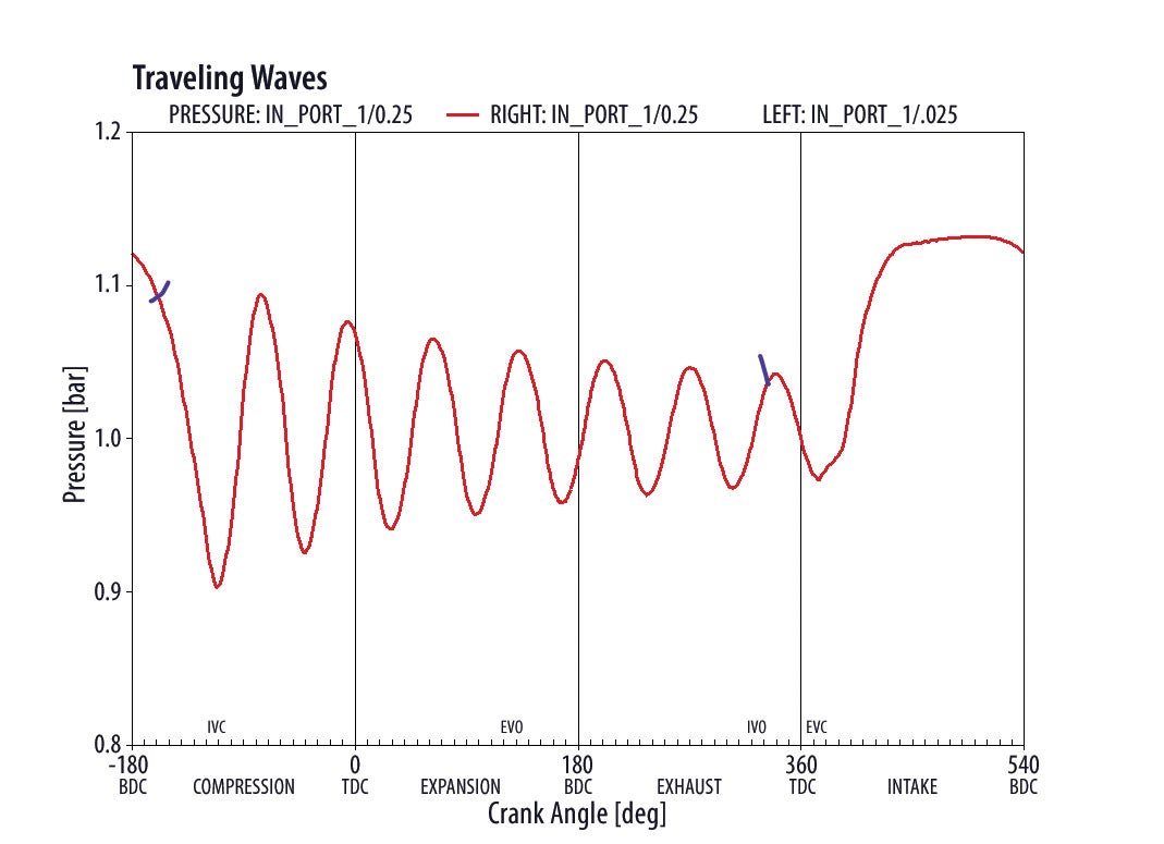
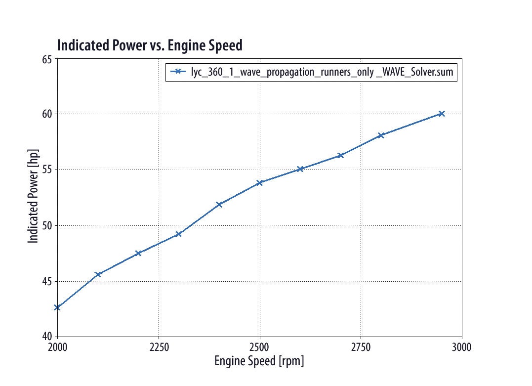
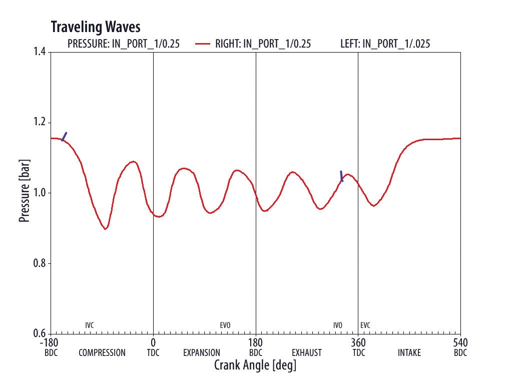
Figure 3 is a graph for a Lycoming single cylinder under “standard conditions” with the optimum runner length. You can see that the proper wave timing comes back into phase at three different rpm positions. These would be the most effective rpm for power or VE (volumetric efficiency) peaking at around 2100, 2400 and 2900 rpm.
The traveling wave diagrams (Figures 4, 5 and 6) represent the optimum positions for wave peaking at each rpm, which are the wave pressures manufactured by Ricardo WAVE at the position of the valve seat. The blue marks indicate pressure at 44.4° BIVC and IVO.
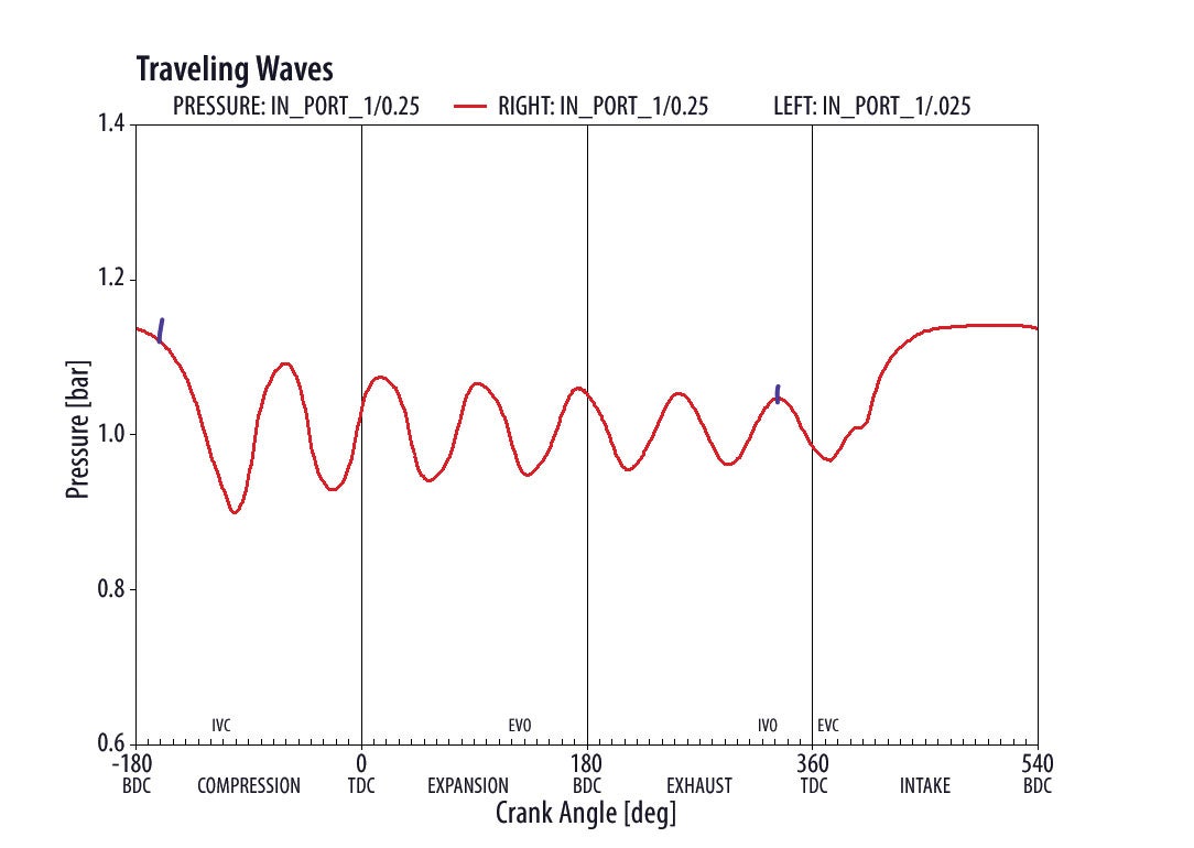
The graphs also show that the N number increases with lower rpm due to the increased time between intake valve events. At 2900 rpm the engine is at the third N between IVO to IVC, which has less attenuation of the wave energy, so there is higher pressure for a more optimum cylinder fill. It appears the tuned plenum with optimum-length runner can increase the power and VE by approximately 7%. That would increase the VE of my engine, which is about 83.7%, to around 91%.
With Ricardo WAVE software we were able to determine the most effective wave timing for highest intake runner pressure to be 44.4° BIVC and intake runner length to be 14.8 inches for our low-rpm engines. It also showed that with a proper runner taper, with an inlet of 2.9 inches tapering to an outlet of 1.685 inches, horsepower output would increase by another 1.25 hp per cylinder; this would add another 2% to the VE.
The current tapered runners from Sky Dynamics added about 1.8 hp per cylinder over non-tapered runners. I was amazed at the ability of this program to even determine optimum runner taper. So it may be possible in the future to have more horsepower while increasing the VE to around 93% by simply bolting on an optimized induction system. I realize that many pilots don’t want to run over 2700 rpm. However, with the tunable induction system you can adjust the runner length to produce the optimum runner pressure to still be at 44.4 degrees BIVC and still increase your horsepower output and optimize its VE, and your engine will have never run smoother.


It’s common knowledge that increasing runner length will move the torque curve toward lower rpms, which is ideal for our slow turning, air cooled engines, but being able to have the taper ratios, etc. being optimized through cascading iterations in Ricardo WAVE sure saves a lot of fabrication effort and risking the engine in incremental trial and error vs. verification of the Ricardo WAVE numbers.
Also, I hope the threaded aluminum sleeves are insulated, either with a layer of glass or kevlar, or a thick layer of Hysol adhesive, from the carbon fiber of the plenum or you’ll be encountering structural failures due to severe corrosion of the sleeves from contact with the carbon.
Comments are closed.